Exploration
Stone Tao
(slides prepared by Hao Su, Quan Vuong, Tongzhou Mu, Zhiao Huang, and Stone Tao)
Spring, 2024
Some contents are based on Bandit
Algorithms from Dr. Tor Lattimore and Prof. Csaba Szepesvári, and COMPM050/COMPGI13 taught at UCL by Prof. David
Silver.
Agenda
Exploration versus Exploitation
Motivation to Explore vs Exploit
- Suppose you go to the same old restauraunt you have been going to for a decade.
- If there is a new restauraunt, do you go and try it? Or do you stick to your priors
- New restauraunt is always a risk (unknown food quality, service etc.)
- But without going to the new restauraunt you never know! How do we balance this?

Why Exploration is Difficult
- Curse of Dimensionality:
- It is common for the state space to be high-dimensional (e.g., image input, multi-joint arms)
- The volume of effective state space grows exponentially w.r.t. dimension!
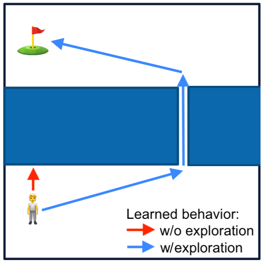
- Even exploration in low-dimensional space may be tricky when there are "alleys". Low probability of going through small gaps to then explore other states:

Exploration to Escape Local Minima in Reward
- Suppose your dense reward for the environment below is euclidean distance to the flag. The return maximizing sequence of actions are to go through the samll gap and reach the flag (global minimum)
- But you will never know to do that unless you explore, and with this dense reward function your trained agent will likely headbutt into the blue wall (local minimum)
Knowing what to explore is critical
- Noisy TV Problem: Imagine an agent encouraged to seek new states to explore. It receives a visual image of what it sees at the moment and needs to explore a maze
- If there was a noisy TV and the agent stumbled upon it, what would happen?
- The agent will become a couch potato and stare at the TV all day.

Balancing Exploration and Exploitation
- Goal: select actions to maximize expected return.
- Problem:
- Actions may have long-term consequences (Credit assignment problem)
- Reward may be delayed (E.g. sparse rewards)
- It may be better to sacrifice immediate reward to gain more long-term reward.
- A high performing policy trade-offs between exploration and exploitation:
- Exploration: take action to learn more about the MDP.
- Exploitation: take the action currently believed to maximize expected return.
Multi-Armed Bandits
Multi-Armed Bandits
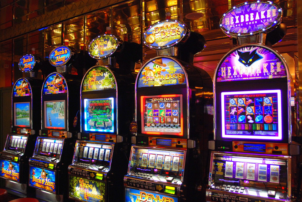
- They are a little bit like a twist on slot machines
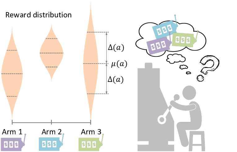
- In this game you have a few slots and can choose a slot to pull. You then receive a reward sampled from an unknown distribution
Multi-Armed Bandits
- A multi-armed bandit is a tuple of action space and reward function $(\mathcal{A}, \mathcal{R})$.
- $\mathcal{A}$ is a finite and known set of actions.
- $\mathcal{R}$ is a function mapping an action to an unknown probability distribution over rewards.
- $\mathcal{R}(a) = \text{Pr} \left[ R | a \right] $
-
At each step $t$, the agent selects an action $a_t$, the environment generates a reward $r_t \sim
Pr[R|a_t]$.
- Note that $a_t$ can be realization of a random variable even if the policy is a deterministic function of input.
- Goal is to maximize cumulative reward $\sum_{t=1}^T r_t$

Regret
- Formal statement about the performance of a policy needs to be made relative to the optimal policy.
- We therefore introduce the notion of regret.
- In general you want to minimize regret
- Think of regret as a form of opportunity cost. The cost of not taking a different action relative to what you did take
- Examples: Investing in stock A vs stock B, taking a trip to Boston vs a trip to New York etc.
Regret (Formalized)
- The action-value of action $a$ is its expected reward: \[ Q(a) = \mathbb{E}_{R}[ R | a ] \]
- The optimal value $V^*$ is the action-value of the optimal action. \[ V^* = Q(a^*) = \operatorname{max}_{a \in \mathcal{A}} Q(a) \]
- The regret of a policy $A_t\sim\pi_t$, where $A_t$ is the distribution of actions the policy generates at time $t$, is the gap between the optimal value and the expected action-value. \[ l_t = V^* - \mathbb{E}_{A_t} \left[ Q(A_t) \right] = \mathbb{E}_{A_t} \left[ V^* - Q(A_t) \right] \]
- The total regret up to time $T$ is the sum of the timestep regret up to time $T$. \[ L_T = \sum_{t=1}^T \mathbb{E}_{A_t} \left[ V^* - Q(A_t) \right] = \mathbb{E}_{A_t} \left[ \sum_{t=1}^T[ V^* - Q(A_t)] \right] \]
- The total regret is sometimes referred to as regret.
Total Regret Decomposition
- The count $N_T(a)$ is the number of times action $a$ was chosen up to time $T$. \[ N_T(a) = \sum_{t=1}^T 1_{A_t = a} \]
- The gap $\Delta_a$ is the difference in value between action $a$ and the optimal action $a^*$. \[ \Delta_a = V^* - Q(a)=V^*-\mathbb{E}_{R} [R|a] \]
- The total regret is a function of gaps and counts. \[ \begin{aligned} L_{T} =\mathbb{E}_{A_t}\left[\sum_{t=1}^{T} [V^{*}-Q\left(A_{t}\right)]\right] =\mathbb{E}_{A_t}\left[\sum_{t=1}^{T} \sum_{a\in\mathcal{A}} 1_{A_t=a}[V^{*}-Q\left(a\right)]\right] =\sum_{a \in \mathcal{A}} \mathbb{E}_{a\sim \pi}\left[N_{T}(a)\right] \Delta_{a} \end{aligned} \]
Total Regret Decomposition
\[ \begin{aligned} L_{T} =\sum_{a \in \mathcal{A}} \mathbb{E}_{a\sim \pi}\left[N_{T}(a)\right] \Delta_{a} \end{aligned} \]- Basic result widely used in regret analysis of bandit algorithms.
- Interpretation? What would an ideal decision making agent do to minimize total regret?
- Interpretation: a good agent picks actions with large gaps less frequently.
- Issue: The gap is not available, since it requires knowing the optimal value $V^*$.
Desirable Total Regret Behavior
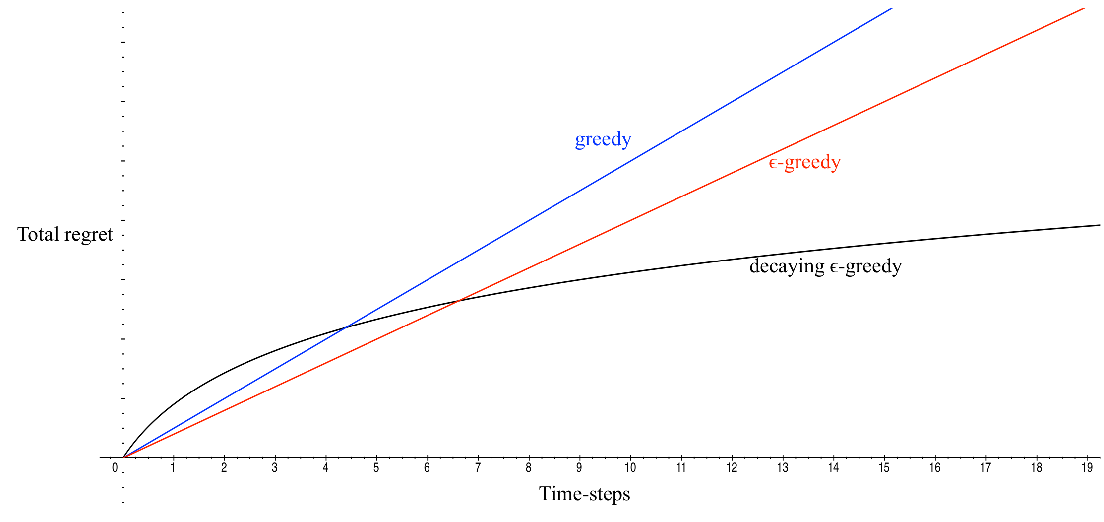
- What can you infer from this figure?
- Ideally, for the total regret, over time:
- the rate of increase quickly decreases
- converge to a small value
- For example, decaying $\epsilon$-greedy (to introduce soon) has logarithmic asymptotic total regret.
Greedy and $\epsilon$-Greedy
- Estimate the value of each action by Monte-Carlo estimation: \[ \hat{Q}_{t}(a)=\frac{1}{N_{t}(a)} \sum_{t'=1}^{t} r_{t'} 1_{A_{t'}=a} \]
- Greedy algorithm selects action with the highest estimated value: \[ a_{t} = \underset{a \in \mathcal{A}} {\operatorname{argmax}} \hat{Q}_{t}(a) \]
- $\epsilon$-Greedy algorithm selects a random action with probability $\epsilon$.
- Both algorithms have linear total regret because Greedy algorithm never explores and $\epsilon$-Greedy algorithm forever explores.
- How to strike a balance? Can we achieve sublinear total regret?
Decaying $\epsilon$-Greedy Algorithm
- By decaying parameter $\epsilon$ in $\epsilon$-Greedy, it is possible to have logarithmic asymptotic total regret.
- Intuitively we are saying to be more confident in our action value estimator Q over time.
- Problem: the decaying schedule requires knowing the gap $\Delta_a = V^* - Q(a), \forall a \in \mathcal{A}$, which is not available.
- How to achieve logarithmic asymptotic total regret without using intractable terms?
The Principle of Optimism in the Face of Uncertainty
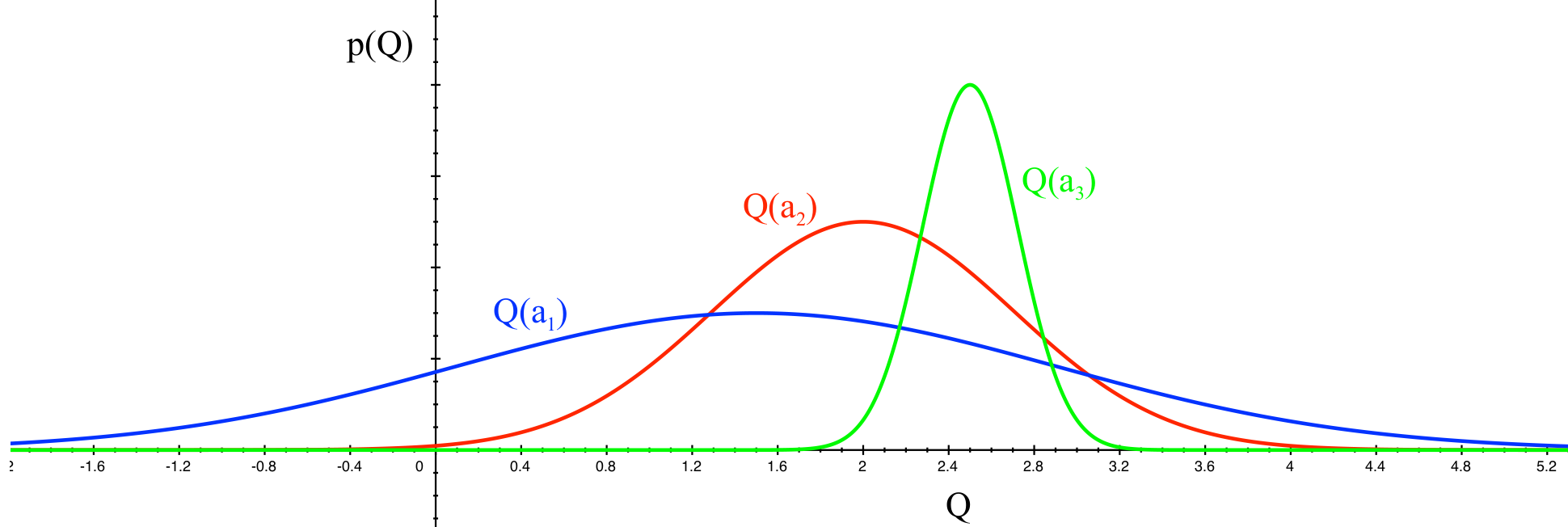
- Given $3$ actions $a_1, a_2, a_3$ with the estimated values as shown.
- Which action should the policy pick to find the optimal action?
- The more uncertain the value estimate of an action is, the more important to take that action.
- In this case, actions $a_1$ and $a_2$ have:
- more uncertain value estimates than $a_3$.
- non-trivial probability of having higher value than $a_3$.
Upper Confidence Bound
-
This principle is operationalized into upper confidence for each action value:
- For each action $a$, estimate an upper confidence $U_t(a)$.
- Such that $Q(a) \leq \hat{Q}_{t}(a)+U_{t}(a)$ with high probability.
- $\hat{Q}_{t}(a)+U_{t}(a)$ is called the Upper Confidence Bound (UCB) of action $a$.
- Select action maximizing the Upper Confidence Bound. \[ a_{t}=\underset{a \in \mathcal{A}}{\operatorname{argmax}} \hat{Q}_{t}(a) + U_{t}(a) \]
Deriving UCB1 Algorithm
- Recall the (weak) law of large numbers: For any positive number $\epsilon$ \[ \lim _{n\to \infty }\Pr \!\left(\,|{\overline {X}}_{n}-\mu |>\varepsilon \,\right)=0 \]
- Interpretation: Empirical average approaches expectation for infinite samples.
- Given finite samples, how far would the empirical average derivate from the expectation?
Deriving UCB1 Algorithm
- Hoeffding's inequality: Let $X_{1}, \ldots, X_{t}$ be i.i.d. random variables in $[0,1]$, and let $\bar{X}_{t}=\frac{1}{t} \sum_{t'=1}^{t} X_{t'}$ be the sample mean. Then: $$ \mathbb{P}\left[\mathbb{E}[X]>\bar{X}_{t}+u\right] \leq e^{-2 t u^{2}} $$
- Applying the inequality to the value estimates of the actions: \[ \mathbb{P}\left[Q(a)>\hat{Q}_{t}(a) + U_{t}(a)\right] \leq e^{-2 N_{t}(a) U_{t}(a)^{2}},\ \forall a\in\mathcal{A} \]
- Assume we know $r_{max}, r_{min}$ for each action and can scale the reward accordingly such that $r \in [0, 1]$.
- Interpretation: $\left[-\infty, \hat{Q}_t(a)+U_{t}(a)\right]$ is the interval that $Q(a)$ will fall in with high probability.
Deriving UCB1 Algorithm
\[\mathbb{P}\left[Q(a)>\hat{Q}_{t}(a) + U_{t}(a)\right] \leq e^{-2 N_{t}(a) U_{t}(a)^{2}}\]- We are interested in finding $U(t)$ so that there is only a small chance that the interval does not cover the true $Q(a)$.
- If the upper bound of this chance is already below $p$, then the interval must be wide enough: \begin{aligned} e^{-2 N_{t}(a) U_{t}(a)^{2}} &\le p \\ \Longrightarrow U_{t}(a) &\ge \sqrt{\frac{-\log p}{2 N_{t}(a)}} \end{aligned}
- Interpretation: $Q(a)$ falls in $\hat{Q}_t(a)+U_{t}(a)$ with probability larger than $1-p$.
- If we would the interval to be tight, then we pick the smallest possible $U_t(a)$.
- Therefore, we take $\hat{Q}_t(a)+\sqrt{\frac{-\log p}{2 N_{t}(a)}}$ as an optimistic estimation of $Q_t(a)$.
Deriving UCB1 Algorithm
- We take $\hat{Q}_t(a)+\sqrt{\frac{-\log p}{2 N_{t}(a)}}$ as an optimistic estimation of $Q_t(a)$.
- To make the numbers concrete, let us assume a decaying $p$ over time: $p = \dfrac{1}{t^4}$. We pick $t^4$ because it eliminates the 2 in the denominator.
- This leads to the UCB1 algorithm: \[ a_{t}=\underset{a \in \mathcal{A}}{\operatorname{argmax}} \hat{Q}_{t}(a) + \sqrt{\frac{2 \log t}{N_{t}(a)}} \]
- Interpretation?
- Interpretation: $N_t(a)$ serves as a proxy for how uncertain the algorithm
- Large $N_t(a)$ $\Longrightarrow$ the policy has taken $N_t(a)$ many times $\Longrightarrow$ Less uncertain value estimate.
- Small $N_t(a)$ $\Longrightarrow$ the policy has not taken $N_t(a)$ many times $\Longrightarrow$ More uncertain value estimate.
- Intuitively we already see the upper bound is logarithmic in time
Theoretical Properties of UCB1 Algorithm
- For any timestep $T$, the total regret of UCB1 is at most logarithmic in the number of timestep $T$: \[ L_T \leq 8 \ln T \underbrace{\left[\sum_{a: \Delta_{a}>0}\left(\frac{1}{\Delta_{a}}\right)\right]}_{const}+\underbrace{\left(1+\frac{\pi^{2}}{3}\right)\left(\sum_{a} \Delta_{a}\right)}_{const} \]
Read by Yourself
Finite-time Analysis of the Multiarmed Bandit Problem. Auer et al.
Intrinsic Rewards
The Perspective of Intrinsic Rewards
- UCB1 chooses actions by estimating an upper confidence for each action value: \[ a_{t}=\underset{a \in \mathcal{A}}{\operatorname{argmax}} \hat{Q}_{t}(a) + \sqrt{\frac{2 \log t}{N_{t}(a)}} \]
- Since we have added a term to $\hat{Q}$, it can be viewed as a reward! We are now encouraging the agent to take actions with the highest upper confidence bounds
- Intrinsic Reward is essentially adding a intrinsic term $i_t$ to the original environment reward $e_t$, giving $r_t = e_t + i_t$
Count Based Exploration
- For small discrete state spaces, we can efficiently count how many times we have visited a state $s$ using a map, let it be $N(s): \mathcal{S} \to \mathbb{Z}$
- What's a simple intrinsic reward you can derive using $N(s)$?
- $r_i=\frac{1}{N(s)}, \frac{1}{N(s)^2}, ...$, basically any function of $N(s)$ that gets smaller as $N(s)$ increases.
Issues with Count Based Exploration
- Impossible for large discrete state spaces. For most $s \in \mathcal{S}$, $N(s)$ is likely 0. For continuous this is impossible
- Very unlikely for agent to visit every state.
- Hence we often look towards pseudo counts, approximations of the actual count.
- Can you think of some simple ways to approximate counts in high dim discrete state spaces? in continuous state spaces?
- Counting via Hashing
- Counting via Density Models
Counting via Hashing
- Come up with some hash function $h : \mathcal{S} \to \mathbb{Z}^k$
- A sort of dimensionality reduction / feature engineering problem
Counting via Hashing: SimHash
- Let $A \in \mathbb{R}^{k \times d}$ with each entry drawn i.i.d from a Gaussian. $g: \mathcal{S} \to \mathbb{R}^{D}$ is a preprocessing function
- $h(s) = \text{sgn}(A g(s)) \in \{-1, 1\}^k$, hashing state $s$ to a sequence of $k$ binary values.
- Drawbacks: Empirically doesn't work for high dimensional observations like images. Deep learning has shown heuristics like simple matrix mappings perform worse than deep neural nets.
Counting via Hashing: Autoencoders
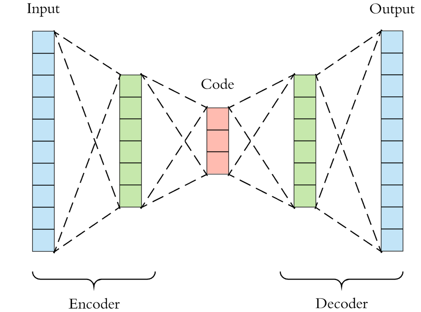
- Autoencoder: Sequence of layers that decrease latent size then increase latent size to reconstruct input
- Trained with a standard reconstruction loss as well as a special augmented loss. $p(s_n)$ is AE output.
- Modifies Autoencoder to include an additional dense layer with K outputs. This dense layer is used for reconstructing the $k$ length binary code from latent state.
- $\mathcal{L}(\{s_n\}_{n=1}^N) = \underbrace{-\frac{1}{N} \sum_{n=1}^N \log p(s_n)}_\text{reconstruction loss} + \underbrace{\frac{1}{N} \frac{\lambda}{K} \sum_{n=1}^N\sum_{i=1}^k \min \big \{ (1-b_i(s_n))^2, b_i(s_n)^2 \big\}}_\text{sigmoid activation being closer to binary}$
Counting via Density Estimation
- Consider a random variable sampled from an arbitrary distribution: \[ X \sim \mathbb{P}(\cdot) \]
- Given samples from the distribution: \[ \{x_1, x_2, \ldots, x_n\} = x_{1:n} \]
- Given an arbitrary sample $x$, the density estimation problem queries the probability of $x$: \[ \mathbb{P}(x | x_{1:n}) \approx \mathbb{P}(x) \]
Density Estimation over State Space
- Consider an MDP $\mathcal{M}$ with a countable state space $\mathcal{S}$, policy $\pi$, denote a sequence of $t$ states by $s_{1:t}$.
- Given $s_{1:t} \sim (\mathcal{M}, \pi)$, a density model over the state space $\mathcal{S}$ is:
\[
\rho_t(s) = \rho(s; s_{1:t}) \approx \mathbb{P}(s | \mathcal{M}, \pi)
\]
- a good density model approximates $\mathbb{P}(s | \mathcal{M}, \pi)$ well
- The empirical density estimation is: \[ \rho_{t}(s) = \frac{N_{t}(s)}{t} \]
- A Gaussian Mixture Model is one density model that can be used which is updated with new data.
Density Estimation over State Space
- Consider an MDP $\mathcal{M}$ with a countable state space $\mathcal{S}$, policy $\pi$, denote a sequence of $t$ states by $s_{1:t}$.
- Given $s_{1:t} \sim (\mathcal{M}, \pi)$, a density model over the state space $\mathcal{S}$ is:
\[
\rho_t(s) = \rho(s; s_{1:t}) \approx \mathbb{P}(s | \mathcal{M}, \pi)
\]
- a good density model approximates $\mathbb{P}(s | \mathcal{M}, \pi)$ well
- Tehe empirical density estimation is: \[ \rho_{t}(s) = \frac{N_{t}(s)}{t} \]
- A Gaussian Mixture Model is one density model that can be used which is updated with new data.
Quick Refresher on GMM
- Gaussian Mixture Model Training Process initializes $k$ different Gaussians and fits them to the data. Suppose for example our state space has 2 dimensions below.
- The GMM is our density model and generates probabilities of seeing some input $p_t(s)$
- Typically optimized via Expectation Maximization (EM)
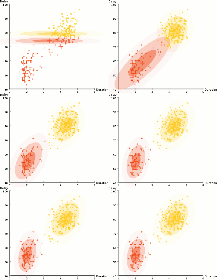
Gif from https://brilliant.org/wiki/gaussian-mixture-model/, which is also a easy resource to learn how EM works.
Computing Pseudo-Count from Density Model
We need to estimate a "pseudo-count" at any state $s$ using a density model $\rho_t(s)$ from visited states $s_{1:t}$. The purpose of the work below is to better "regulate" the density model and make it possible to get pseudo-counts from any density model.- First, given $s_{1:t}$, we can estimate the density of some state $s$ by \[ \rho_t(s)=\rho(s;s_{1:t}) \]
- Next, we "imagine" that next step we will obtain one more sample of $s$, i.e., the visited state sequence becomes $\{s_{1:t}, s\}$. Then, the density of $s$ will be \[ \rho_{t+1}(s) = \rho( s; s_{1:t}, s ) \]
Computing Pseudo-Count from Density Model
- According to the empirical density estimation formula, we "expect" that the pseudo count of state visitation $\hat{N}_t$ to satisify \[ \rho_{t}(s) = \frac{\hat{N}_{t}(s)}{t}, \quad \quad \rho_{t+1}(s) = \frac{\hat{N}_{t}(s)+1}{t+1} \]
- Cancel $t$ from the equations, and we can solve $\hat{N}_t(s)$: \[ \hat{N}_{t}(s)=\frac{\rho_{t}(s)\left(1-\rho_{t+1}(s)\right)}{\rho_{t+1}(s)-\rho_{t}(s)} \]
- The new MDP reward function with hyperparameters $\beta$ and $\epsilon$ (paper uses $\epsilon = 0.01, \beta =1$) is: \[ R(x, a) + \sqrt{\frac{\beta}{\hat{N}_{t}(s)+\epsilon}} \]
Pseudo-Count Performance
- Observations are images. Actions are move left, right, jump, go down.
-
In $100$ million frames of training:
- DQN explores $2$ rooms
- DQN + pseudo-count explores $15$ different rooms
- Go to 1:50 mark in the video to see exploration behavior.
Intrinsic Rewards
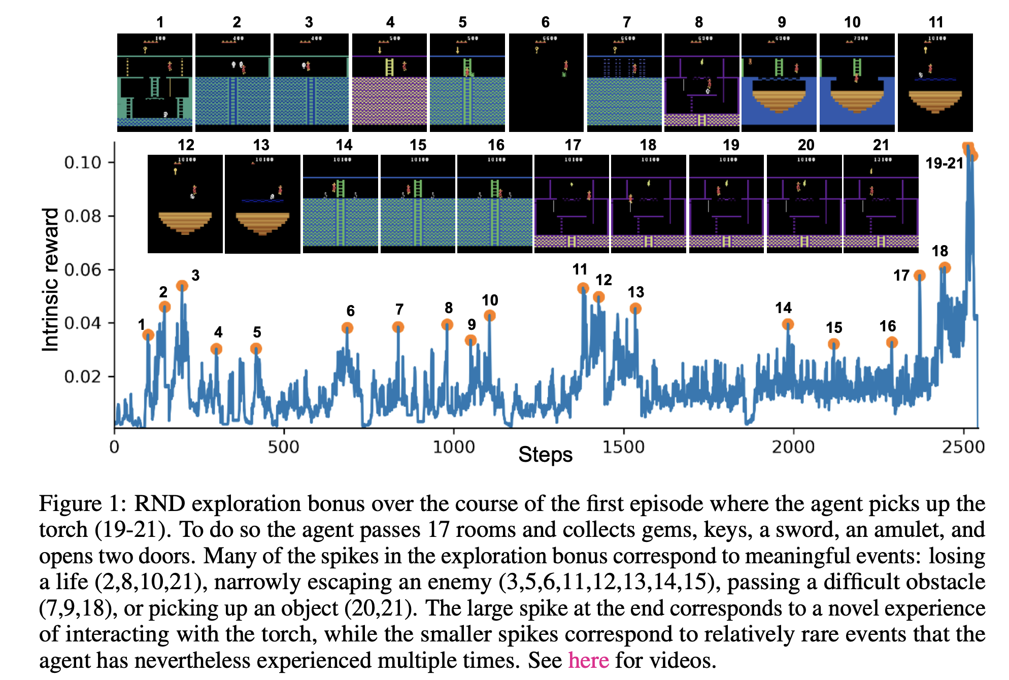
- In addition to the pseudo-count, there are many other ways to compute an intrinsic reward:
- Random Network Distillation
- Curiosity-driven exploration through:
- forward dynamics prediction model
- inverse dynamics model
- Entropy regularization
- etc ...
- Generally we want to encourage taking actions to reach novel states we have not seen before and should see
Leveraging Model Predicton Errors for Novelty
- Suppose you train a neural net to predict the MDP dynamics function $\rho : \mathcal{S} \times \mathcal{A} \to \mathcal{S}$. Predict $s_{t+1} = \rho(s_t, a)$ (training a world model). Intuitively if we can't predict the next state, then the current state is one that needs more data collection/exploration
- When might the trained neural net fail to predict the next state accurately? And which errors can be used for intrisnic rewards?
- Lack of seen training data (similar to count based exploration!). Also known as epistemic uncertainty
- Stochastic Environment States (hard to predict with any function when the data itself is not determinstic). Also known as aleatoric uncertainty
- Model misspecification. Perhaps some critical data that makes an MDP markov was not given to the model, or the model architecture / function structure itself is not sufficiently expressive.
- Only error due to lack of training data can be used. All else is pure noise that will be hard to learn from. We will introduce Random network Distillation and see how that helps.
Random Network Distillation (RND)
- Use two neural networks to compute the novelty bonus (intrinsic reward $i_t$):
- A fixed and randomly initialized target network, mapping observation to $k$-dim features, $f: \mathcal{S} \rightarrow \mathbb{R}^{k}$
- A predictor network, $\hat{f}_{\theta}: \mathcal{S} \rightarrow \mathbb{R}^{k}$
- Given a state $s_t$, the novelty bonus is the difference in predicted features. \[ i_t = \| \hat{f}_\theta(s_t) - f(s_t) \|^2 \]
- The predictor network is trained to match the output of the target network using previously collected experience: \[ \text{minimize}_{\theta} \| \hat{f}_{\theta}(s) - f(s) \|^2 \] Usually we only optimize for a few steps (with e.g. MSE loss).
RND Intuition
- Which of the prediction errors below does RND have and why?
- Lack of seen training data: RND has this type of error, it is when $\hat{f}_\theta$ has not been trained enough (seen enough samples) on data to predict target neural net $f$ output
- Stochastic Environment States: RND does not have this type of error. The target prediction is another neural net $f$ that is deterministic
- Model misspecification: RND "generally" does not have this error. The targets $\hat{f}_\theta$ must predict are generated by a neural network with the same inputs and architecture.
- We see that RND has some nice properties for intrinsic reward generation! We will now see it in practice next
Summary of Terms
- Credit Assignment Problem: Figuring out how much an action influenced our reward/return
- Noisy TV Problem: A problem when an agent seeking novel states gets stuck exploring the wrong novel states (like a noisy tv).
- Multi-Armed Bandit Problem: Repeatedly select 1 of K levers and receive a reward sampled from the lever's distribution.
- Regret: Optimal action's reward minus achieved reward. Similar to opportunity cost.
- Upper Confidence Bound: A upper bound on the optimal value of an action with logarithmic scale regret.
- Intrinsic Reward: An additional reward added to an environment (extrinsic) reward.
- Epistemic Uncertainty: The uncertainty associated with randomness that can be explained/predicted (when given suffficient information)
- Aleatoric Uncertainty: The uncertainty associated with randomness that cannot be explained/predicted
