Agenda

click to jump to the section.

Optimal Value Function

• Due to the Markovian property, the return starting from a state $s$ is independent of its history. Therefore, we can compare the return of all policies starting from $s$ and find the optimal one.
• The optimal state-value function $V^*(s)$ is the maximum value function over all policies
  • $V^*(s)=\max_\pi V_\pi(s)$
• The optimal action-value function $Q_*(s,a)$ is the maximum action-value function over all policies
  • $Q^*(s,a)=\max_\pi Q_\pi(s,a)$
• The optimal value function specifies the best possible performance in the MDP.

Optimal Policy

• Define a partial ordering over policies \[ \pi\ge\pi'\mbox{ if }V_\pi(s)\ge V_{\pi'}(s), \forall s \]

Theorem: For any Markov Decision Process

• There exists an optimal policy $\pi_*$ that is better than, or equal to, all other policies, $\pi_*\ge\pi,~\forall\pi$
• All optimal policies achieve the optimal value function, $V_{\pi^*}(s)=V^*(s)$
• All optimal policies achieve the optimal action-value function, $Q_{\pi^*}(s,a)=Q^*(s,a)$

• An optimal policy can be found by maximizing over $Q^*(s,a)$, \[ \pi^*(a|s)= \begin{cases} 1, & \text{if}~~a=\text{argmax}_{a\in\mc{A}}~Q^*(s,a) \\ 0, & \text{otherwise} \end{cases} \]

Bellman Optimality Equation

• Optimal value functions also satisfy recursive relationships \[ \begin{aligned} V^*(s) & = \max_a Q^*(s,a) \\ & = \max_a\bb{E}_{\pi_*}[G_t|S_t=s, A_t=a] \\ & = \max_a\bb{E}_{\pi_*}[R_{t+1}+\gamma G_{t+1}|S_t=s, A_t=a] \\ & = \max_a\bb{E}[R_{t+1}+\gamma V^*(S_{t+1})|S_t=s, A_t=a] \\ \end{aligned} \]
• Similarly, for action-value function, we have
\[ Q^*(s,a)=\bb{E}[R_{t+1}+\gamma \max_{a'}Q^*(S_{t+1}, a')|S_t=s, A_t=a] \]
• They are called Bellman Optimality Equations

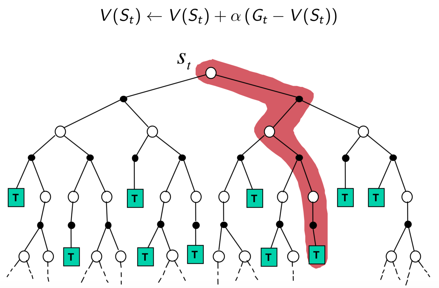
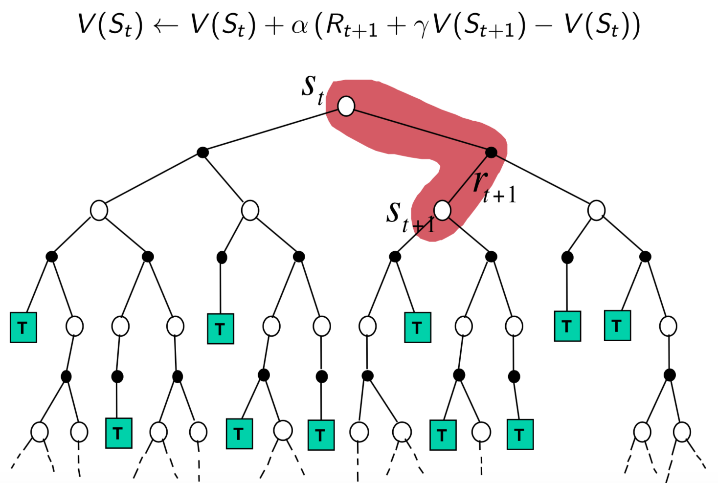
Key Differences between MC and TD

• MC estimates values based on rollout
• TD estimates values based on Bellman equation

Pros and Cons of MC vs TD (2)

• MC has high variance, zero bias
  • Good convergence properties (even with function approximation)
  • Independent of the initial value of $V$
  • Very simple to understand and use
• TD has low variance, some bias
  • Usually more efficient than MC
  • TD(0) converges to $V_\pi(s)$ (but not always with function approximation)
  • Has certain dependency on the initial value of $V$

The Anatomy of an RL algorithm

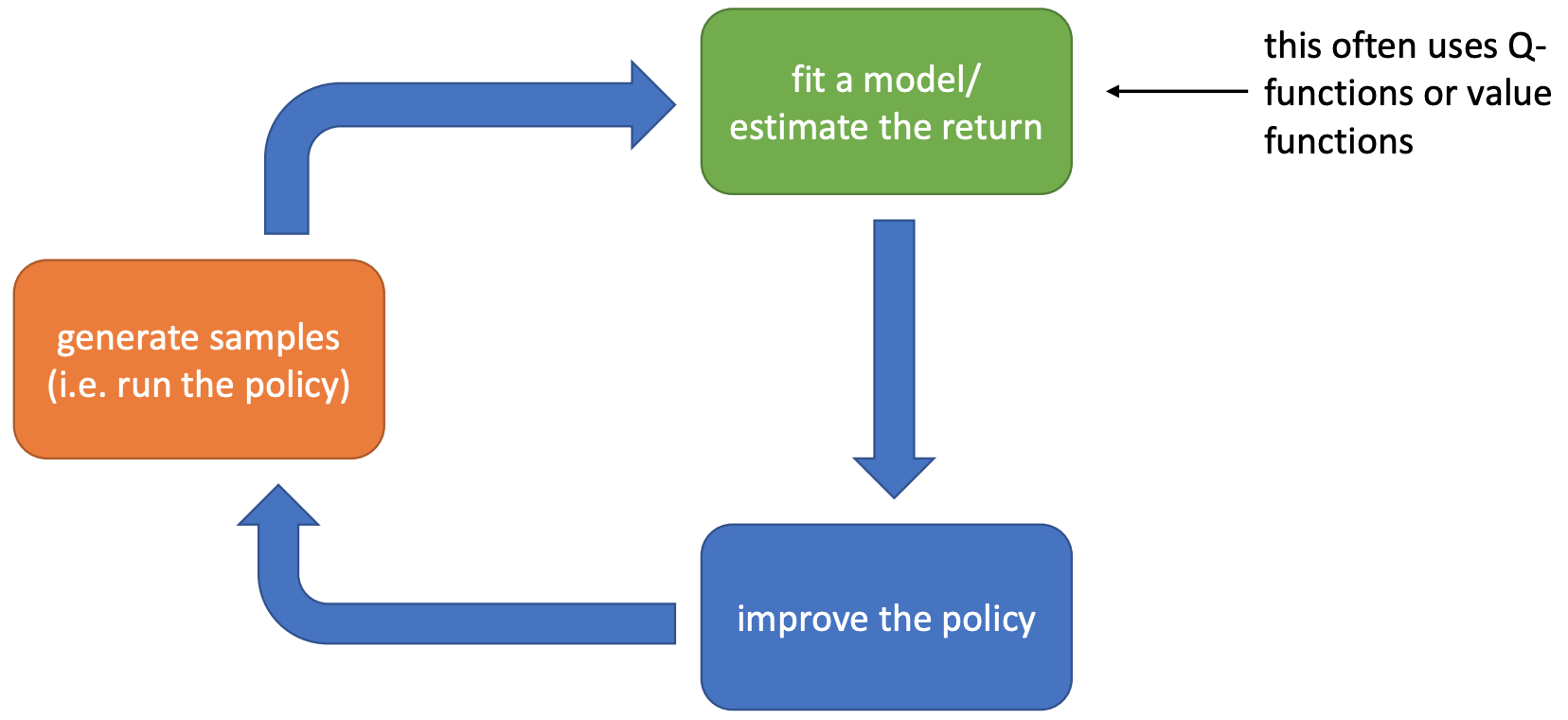
• Suppose we are going to learn the Q-function. Let us follow the previous flow chart and answer three questions:
1. Given transitions $\{(s,a,s',r)\}$ from some trajectories, how to update the current Q-function?
   • By Temporal Difference learning, the update target for $Q(S,A)$ is
     • $R+\gamma\max_a Q(S', a)$
   • Take a small step towards the target
     • $Q(S,A)\leftarrow Q(S,A)+\alpha[R+\gamma\max_a Q(S', a)-Q(S,A)]$
2. Given $Q$, how to improve policy?
   • Take the greedy policy based on the current $Q$
     • $\pi(s)=\text{argmax}_a Q(s,a)$
3. Given $\pi$, how to generate trajectories?
   • Run the $\epsilon$-greedy policy in the environment.

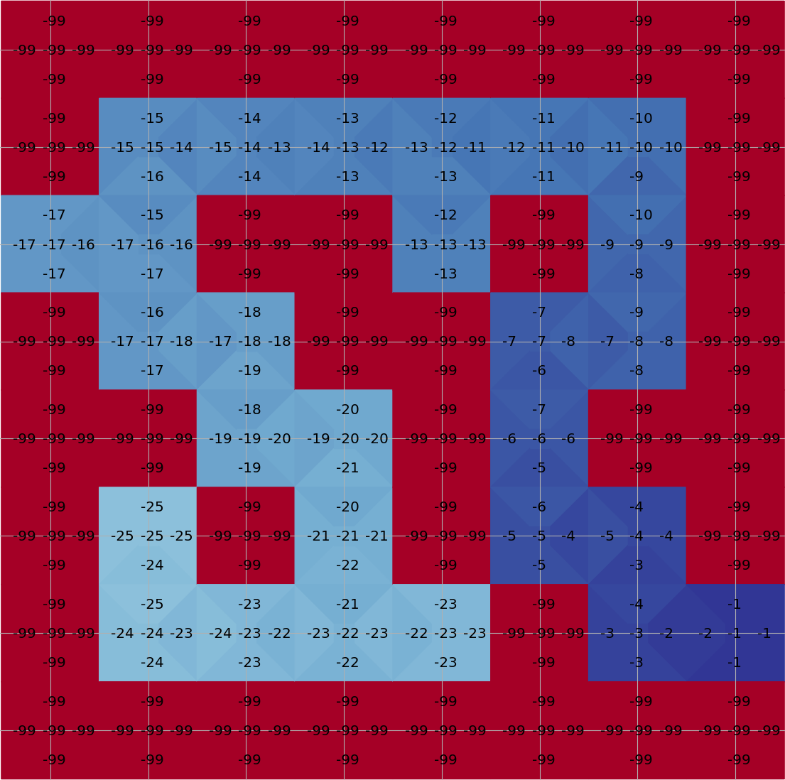
Running Q-learning on Maze

Taxonomy of RL Algorithms and Examples

Challenge of Representing $Q$

• How do we represent $Q(s,a)$?
• Maze has a discrete and small state space that we can deal with by an array.
• However, for many cases the state space is continuous, or discrete but huge, array does not work.

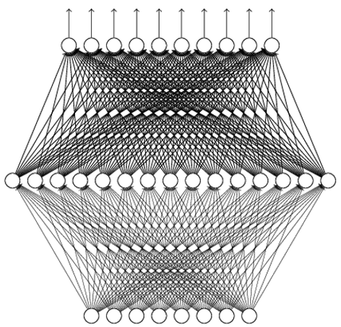
Deep Value Network

• Use a neural network to parameterize $Q$:
• Input: state $s\in\bb{R}^n$
• Output: each dimension for the value of an action $Q(s, a;\theta)$

Training Deep Q Network

• Recall the Bellman optimality equation for action-value function: \[ Q^*(s,a)=\bb{E}[R_{t+1}+\gamma \max_{a'}Q^*(S_{t+1}, a')|S_t=s, A_t=a] \]
• It is natural to build an optimization problem: \[ L(\th)=\bb{E}_{\color{red}{(s,a,s',r)\sim Env}}[TD_{\th}(s,a,s',r)] \tag{TD loss} \] where $TD_{\th}(s,a,s',r)=\|Q_{\th}(s,a)-[r+\gamma\max_{a'}Q_{\th}(s',a')]\|^2$.
• Note: How to obtain the $Env$ distribution has many options!
  • It does not necessarily sample from the optimal policy.
  • A suboptimal, or even bad policy (e.g., random policy), may allow us to learn a good $Q$.
  • It is a cutting-edge research topic of studying how well we can do for non-optimal $Env$ distribution.

Replay Buffer

• As in the previous Q-learning, we consider a routine that we take turns to
• Sample certain transitions using the current $Q_{\th}$
• Update $Q_{\th}$ by minimizing the TD loss
• Collecting data:
  • We use $\epsilon$-greedy strategy to sample transitions, and add $(s,a,s',r)$ in a replay buffer (e.g., maintained by FIFO).
• Updating Q:
  • We sample a batch of transitions and train the network by gradient descent: \[ \nabla_{\th}L(\th)=\bb{E}_{(s,a,s',r)\sim \rm{Replay Buffer}}[\nabla_{\th}TD_{\th}(s,a,s',r)] \]

Deep Q-Learning Algorithm

• Initialize the replay buffer $D$ and Q network $Q_{\th}$.
• For every episode:
  • Sample the initial state $s_0\sim P(s_0)$
  • Repeat until the episode is over
    • Let $s$ be the current state
    • With prob. $\epsilon$ sample a random action $a$. Otherwise select $a=\arg\max_a Q_{\th}(s,a)$
    • Execute $a$ in the environment, and receive the reward $r$ and the next state $s'$
    • Add transitions $(s,a,s',r)$ in $D$
    • Sample a random batch from $D$ and build the batch TD loss
    • Perform one or a few gradient descent steps on the TD loss

Some Engineering Concerns about
Deep $Q$-Learning

• States and value network architecture
• First of all, a good computer vision problem worth research.
• Need to ensure that states are sufficient statistics for decision-making
  • Common practice: Stack a fixed number of frames (e.g., 4 frames) and pass through ConvNet
  • If long-term history is important, may use LSTM/GRU/Transformer/... to aggregate past history
• May add other computing structures that are effective for video analysis, e.g., optical flow map
• Not all vision layers can be applied without verification (e.g., batch normalization layer may be harmful)
• Replay buffer
• Replay buffer size matters.
• When sampling from the replay buffer, relatively large buffer size helps stabilizing training.

Some Theoretical Concerns about $Q$-Learning

• Behavior/Target Network: Recall that $TD_{\th}(s,a,s',r)=\|\color{blue}{Q_{\th}(s,a)}-[r+\gamma\max_{a'}\color{red}{Q_{\th}(s',a')}]\|^2$. We keep two $Q$ networks in practice. We only update the blue network by gradient descent and use it to sample new trajectories. Every few episodes we replace the red one by the blue one. The reason is that the blue one changes too fast. The red one is called target network (to build target), and the blue one is called behavior network (to sample actions).
• Value overestimation: Note that the TD target takes the maximal $a$ for each $Q(s,\cdot)$. Since TD target can be biased, the max operator will cause the $Q$-value to be overestimated! There are methods to mitigate (e.g., double Q-learning) or work around (e.g., advantage function) the issue.
• Uncertainty of $Q$ estimation: Obviously, the $Q$ value at some $(s,a)$ are estimated from more samples, and should be more trustable. Those high $Q$ value with low confidence are quite detrimental to performance. Distributional Q-Learning quantifies the confidence of $Q$ and leverages the confidence to recalibrate target values and conduct exploration.

Convergence of Q-Learning Algorithms

We state the facts without proof:

• Q-Learning:
  • Tabular setup: Guaranteed convergence to the optimal solution. A simple proof (using contraction mapping).
  • Value network setup: No convergence guarantee due to the approximation nature of networks.

Taxonomy of RL Algorithms and Examples

First-Order Policy Optimization

• Recall that a policy $\pi$ (assume its independent of step $t$) is just a function that maps from a state to a distribution over the action space.
  • The quality of $\pi$ is determined by $V^{\pi}(s_0)$, where $s_0$ is the initial state
    • Q: What if the initial state is a distribution?
  • We can parameterize $\pi$ by $\pi_{\theta}$, e.g.,
    • a neural network
    • a categorical distribution

First-Order Policy Optimization

• Now we can formulate policy optimization as \[ \begin{align} \underset{\theta\in\Theta}{\text{maximize}}&&V^{\pi_{\theta}}(s_0). \end{align} \]

• Sampling allows us to estimate values.
• If sampling also allows us to estimate the gradient of values w.r.t. policy parameters $\frac{\partial V^{\pi_{\theta}}(s_0)}{\partial \theta}$, we can improve our policies!

Goal: Derivate a way to directly estimate the gradient $\frac{\partial V^{\pi_{\theta}}(s_0)}{\partial \theta}$ from samples.

Policy Gradient Theorem (Undiscounted)

• By Bellman expectation equation, \begin{align*} V^{\pi_{\theta}}(s) &= \bb{E}_{\pi_{\theta}} [R_{t+1}+ V_{\pi}(S_{t+1})|S_t=s]\\ &=\sum_{a}\pi_{\theta}(a|s)\cdot\mathbb{E}_{s'\sim T(s, a)}\left[r(s, a) + V^{\pi_{\theta}}(s')\right]. \end{align*}
• How to calculate $\nabla_{\theta}V^{\pi_{\theta}}(s_0)$? Note that, \begin{align*} \nabla_{\theta}V^{\pi_{\theta}}(s_0) &= \sum_{a_0}\nabla_{\theta}\left\{\pi_{\theta}(a_0|s_0)\cdot\mathbb{E}_{s_1\sim T(s_0, a_0)}\left[r(s_0, a_0) + V^{\pi_{\theta}}(s_1)\right]\right\}\\ \text{(product rule)} &= \sum_{a_0} \left\{ \nabla_{\theta}\pi_{\theta}(a_0|s_0) \cdot \mathbb{E}_{s_1\sim T(s_0, a_0)}\left[r(s_0, a_0) + V^{\pi_{\theta}}(s_1)\right] + \pi_{\theta}(a_0|s_0)\cdot \mathbb{E}_{s_1\sim T(s_0, a_0)}\left[\nabla_{\theta}V^{\pi_{\theta}}(s_1)\right] \right\}\\ &= \sum_{a_0} \left\{ \nabla_{\theta}\pi_{\theta}(a_0|s_0) \cdot Q^{\pi_{\theta}}(s_0, a_0) + \pi_{\theta}(a_0|s_0)\cdot \mathbb{E}_{s_1\sim T(s_0, a_0)}\left[\sum_{a_1}\{\nabla_{\theta}\pi_{\theta}(a_1|s_1)Q^{\pi_{\theta}}(s_1,a_1)+ \pi_{\theta}(a_1|s_1)\bb{E}[\nabla_{\theta}V^{\pi_{\theta}}(s_2)]\}\right] \right\}\\ &=\left\{\sum_{a_0} \nabla_{\theta}\pi_{\theta}(a_0|s_0) \cdot Q^{\pi_{\theta}}(s_0, a_0)\right\} + \left\{\sum_{a_0}\pi_{\theta}(a_0|s_0)\cdot \mathbb{E}_{s_1\sim T(s_0, a_0)}\left[\sum_{a_1}\nabla_{\theta}\pi_{\theta}(a_1|s_1)Q^{\pi_{\theta}}(s_1,a_1)\right]\right\} + ... \\ \text{(recursively repeat above)} &= \sum_{t = 0}^{\infty}\sum_s\mu_t(s;s_0) \sum_{a}\nabla_{\theta}\pi_{\theta}(a|s) \cdot Q^{\pi_{\theta}}(s, a)=\sum_{s}\sum_t^{\infty}\mu_t(s;s_0) \sum_{a}\nabla_{\theta}\pi_{\theta}(a|s) \cdot Q^{\pi_{\theta}}(s, a) \end{align*} Q: What does $\mu_t(s;s_0)$ mean?

Policy Gradient Theorem (Undiscounted)

• Policy Gradient Theorem (Undiscounted): \[ \nabla_{\theta}V^{\pi_{\theta}}(s_0)=\sum_{s}\sum_t^{\infty}\mu_t(s;s_0) \sum_{a}\nabla_{\theta}\pi_{\theta}(a|s) \cdot Q^{\pi_{\theta}}(s, a) \] where $\mu_t(s;s_0)$ is the average visitation frequency of the state $s$ in step $t$, and $\sum_s \mu_t(s;s_0)=1$.
• Q: What is the intuitive interpretation from this equation?
  • Weighted sum of (log) policy gradients for all steps.
  • Higher weights for states with higher frequency.

Policy Gradient Theorem (Discounted)

• Policy Gradient Theorem (Discounted): \[ \nabla_{\th}V^{\pi_{\theta, \gamma}}(s_0) = \sum_s\sum_{t = 0}^{\infty}\gamma^t\mu_t(s;s_0) \sum_{a}\nabla_{\theta}\pi_{\theta}(a|s) \cdot Q^{\pi_{\theta}, \gamma}(s, a). \] $\mu_t(s;s_0)$ is the average visitation frequency of the state $s$ in step $t$.
• Can you guess the influence of $\gamma$ in this result?

We will assume the discounted setting from now on.

Creating an Unbiased Estimate for PG

\[ \nabla_{\theta}V^{\pi_{\theta}, \gamma}(s_0) =\sum_{t = 0}^{\infty}\sum_s\gamma^t\mu_t(s;s_0) \sum_{a}\nabla_{\theta}\pi_{\theta}(a|s) \cdot Q^{\pi_{\theta}, \gamma}(s, a) \] Let's say we have used $\pi_{\theta}$ to collect a rollout trajectory $\left\{(s_t, a_t, r_t)\right\}_{t = 0}^{\infty}$, where $s_t, a_t, r_t$ are random variables. Note that $\nabla_{\th} \ln \pi_{\th}=\frac{\nabla \pi_{\th}}{\pi_{\th}}\Rightarrow \nabla \pi_{\th}=\nabla_{\theta} \ln(\pi_{\th})\cdot\pi_{\th}$ \begin{align*} \nabla_{\theta}V^{\pi_{\theta}, \gamma}(s_0)&= \sum_s\sum_{t = 0}^{\infty}\gamma^t\mu_t(s;s_0)\sum_{a}\nabla_{\theta}\ln\left(\pi_{\theta}(a|s)\right) \cdot \pi_{\theta}(a|s) Q^{\pi_{\theta}, \gamma}(s, a)\\ \text{(absorb randomness of env. in $\mu_t$)} &=\mathbb{E}\left[\sum_{t = 0}^{\infty}\gamma^t\sum_{a}\nabla_{\theta}\ln\left(\pi_{\theta}(a|s_t)\right)\cdot\pi_{\theta}(a|s_t)Q^{\pi_{\theta}, \gamma}(s_t, a)\right]\\ \text{(absorb randomness of action in $\pi_{\th}$)}&=\mathbb{E}\left[\sum_{t = 0}^{\infty}\gamma^t\nabla_{\theta}\ln\left(\pi_{\theta}(a_t|s_t)\right)\cdot Q^{\pi_{\theta}, \gamma}(s_t, a_t)\right]\\ &=\mathbb{E}\left[\sum_{t = 0}^{\infty}\gamma^t\nabla_{\theta}\ln\left(\pi_{\theta}(a_t|s_t)\right)\cdot \sum_{i = t}^{\infty} \gamma^{i - t}\cdot r_i\right]\\ \end{align*}

Creating an Unbiased Estimate for PG (Cont'd)

We have shown that \begin{align*} \nabla_{\theta}V^{\pi_{\theta}, \gamma}(s_0)=\mathbb{E}\left[\sum_{t = 0}^{\infty}\gamma^t\nabla_{\theta}\ln\left(\pi_{\theta}(a_t|s_t)\right)\cdot \sum_{i = t}^{\infty} \gamma^{i - t}\cdot r_i\right]\\ \end{align*}

• Using more trajectories, we can get more accurate gradient estimate (smaller variance)
• Since the unbiased estimate is a summation, we can sample from the individual terms to do batched gradient descent

We have established an MC sampling based method to
estimate the gradient of value w.r.t. policy parameters!
This estimate is unbiased.

• In literature, this MC-sampling based policy gradient method is called REINFORCE.

REINFORCE Algorithm

The steps involved in the implementation of REINFORCE would be as follows:

1. Randomly initialize a policy network that takes the state as input and returns the probability of actions
2. Use the policy to play $n$ episodes of the game. Record $(s,a,s',r)$ for each step.
3. Calculate the discounted reward for each step backwards
4. Calculate expected reward $G_t=\sum_{i=t}^{\infty}\gamma^{i-t}r_i$
5. Adjust weights of policy according to the gradient by policy gradient theorem
6. Repeat from 2

Difference between Theory and Practice

According to what we have derived from the Policy Gradient Theorem (discounted): \begin{align*} \nabla_{\theta}V^{\pi_{\theta}, \gamma}(s_0)=\mathbb{E}\left[\sum_{t = 0}^{\infty}\gamma^t\nabla_{\theta}\ln\left(\pi_{\theta}(a_t|s_t)\right)\cdot \sum_{i = t}^{\infty} \gamma^{i - t}\cdot r_i\right]\\ \end{align*} However, in the practical REINFORCE algorithm implementation, we use \begin{align*} \nabla_{\theta}V^{\pi_{\theta}, \gamma}(s_0)=\mathbb{E}\left[\sum_{t = 0}^{\infty}\nabla_{\theta}\ln\left(\pi_{\theta}(a_t|s_t)\right)\cdot \sum_{i = t}^{\infty} \gamma^{i - t}\cdot r_i\right]\\ \end{align*} See the following articles for further discussions:

• Is the Policy Gradient a Gradient?
• Why there is a problem with the Policy Gradient theorem in Deep Reinforcement Learning

End