L3: Framework of Reinforcement Learning (II)
Tongzhou Mu
(slides prepared by Hao Su and Tongzhou Mu)
Spring, 2024
Contents are based on Reinforcement Learning: An Introduction from Prof. Richard S. Sutton and Prof. Andrew G. Barto, and COMPM050/COMPGI13 taught at UCL by Prof. David Silver.
Agenda
Review
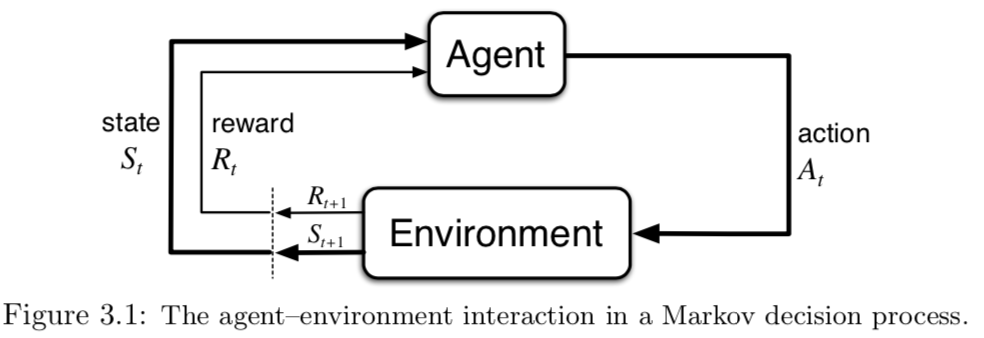
Agent-Environment Interface
- Agent: learner and decision maker.
- Environment: the thing agent interacts with, comprising everything outside the agent.
- Action: how agent interacts with the environment.
- In engineers’ terms, they are called controller, controlled system (or plant), and control signal.
Probabilistic Description of Environment: Markov Decision Processes
- A Markov decision process (MDP) is a Markov process with rewards and decisions.
- Definition:
- A Markov decision process is a tuple $(\mc{S}, \mc{A}, \mc{P}, \mc{R})$
- $\mc{S}$ is a set of states (discrete or continuous)
- $\mc{A}$ is a set of actions (discrete or continuous)
- $\mc{P}$ is a state transition probability function
- $\mc{P}^{a}_{s,s'}=P(s'|s,a)=\text{Pr}(S_{t+1}=s'|S_t=s,A_t=a)$
- $\mc{R}$ is a reward function
- $\mc{R}^{a}_{s}=R(s,a)=\bb{E}[R_{t+1}|S_t=s,A_t=a]$
- Sometimes, an MDP also includes an initial state distribution $\mu$
Policy
- A policy is the agent's behaviour
- It is a map from state to action, e.g.,
- Deterministic policy: $a=\pi(s)$
- Stochastic policy: $\pi(a|s)=\text{Pr}(A_t=a|S_t=s)$
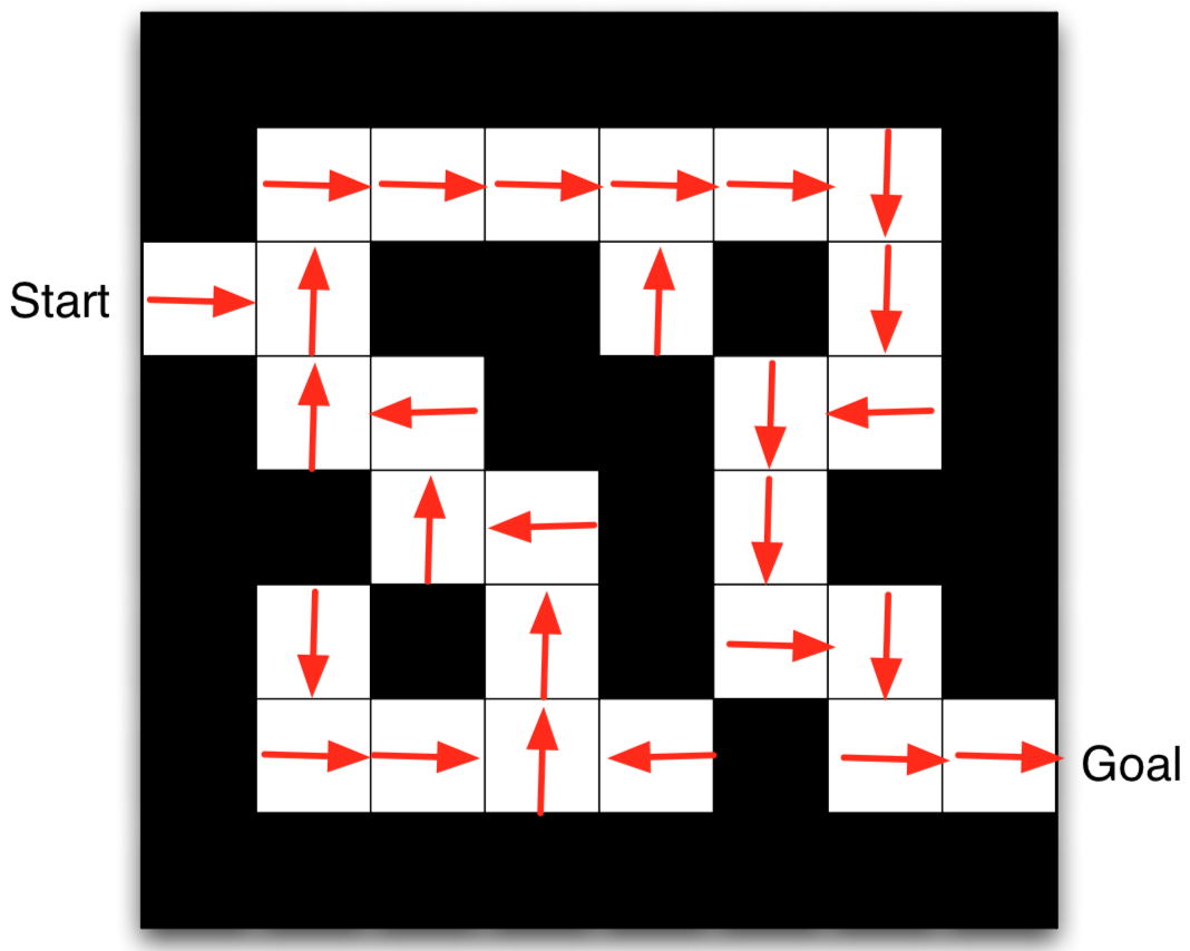
Maze Example: Policy
- Arrows represent policy $\pi(s)$ for each state s
- This is the optimal policy for this Maze MDP
Value Function
- Value function is a prediction of future reward
- Evaluates the goodness/badness of states
- State-value function
- The state-value function $V_\pi(s)$ of an MDP is the expected return starting from state $s$, following the policy $\pi$
- $V_\pi(s)=\bb{E}_\pi[G_t|S_t=s]$ (assuming infinite horizon here)
- Action-value function
- The action-value function $Q_\pi(s,a)$ is the expected return starting from state $s$, taking action $a$, following policy $\pi$
- $Q_\pi(s,a)=\bb{E}_\pi[G_t|S_t=s, A_t=a]$ (assuming infinite horizon here)
- Notation explanation:
- In this lecture, when we write $\bb{E}_\pi$, it means we take expectation over all samples/trajectories generated by running the policy $\pi$ in the environment
- So it counts for all the randomness from policy, initial state, state transition, and reward.
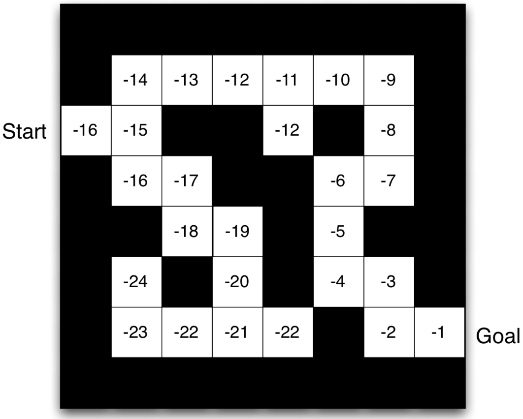
Maze Example: Value Function
- Numbers represent value $V_\pi(s)$ of each state $s$
- This is the value function corresponds to the optimal policy we showed previously
Optimal Policy and Optimal Value Function
Optimal Value Function
- Due to the Markovian property, the return starting from a state $s$ is independent of its history. Therefore, we can compare the return of all policies starting from $s$ and find the optimal one.
- The optimal state-value function $V^*(s)$ is the maximum value function over all policies
- $V^*(s)=\max_\pi V_\pi(s)$
- The optimal action-value function $Q_*(s,a)$ is the maximum action-value function over all policies
- $Q^*(s,a)=\max_\pi Q_\pi(s,a)$
- The optimal value function specifies the best possible performance in the MDP.
Optimal Policy
- Define a partial ordering over policies \[ \pi\ge\pi'\mbox{ if }V_\pi(s)\ge V_{\pi'}(s), \forall s \]
- There exists an optimal policy $\pi_*$ that is better than, or equal to, all other policies, $\pi_*\ge\pi,~\forall\pi$
- All optimal policies achieve the optimal value function, $V_{\pi^*}(s)=V^*(s)$
- All optimal policies achieve the optimal action-value function, $Q_{\pi^*}(s,a)=Q^*(s,a)$
- An optimal policy can be found by maximizing over $Q^*(s,a)$, \[ \pi^*(a|s)= \begin{cases} 1, & \text{if}~~a=\text{argmax}_{a\in\mc{A}}~Q^*(s,a) \\ 0, & \text{otherwise} \end{cases} \]
Theorem: For any Markov Decision Process
Bellman Optimality Equation
- Optimal value functions also satisfy recursive relationships \[ \begin{aligned} V^*(s) & = \max_a Q^*(s,a) \\ & = \max_a\bb{E}_{\pi_*}[G_t|S_t=s, A_t=a] \\ & = \max_a\bb{E}_{\pi_*}[R_{t+1}+\gamma G_{t+1}|S_t=s, A_t=a] \\ & = \max_a\bb{E}[R_{t+1}+\gamma V^*(S_{t+1})|S_t=s, A_t=a] \\ \end{aligned} \]
- Similarly, for action-value function, we have \[ Q^*(s,a)=\bb{E}[R_{t+1}+\gamma \max_{a'}Q^*(S_{t+1}, a')|S_t=s, A_t=a] \]
- They are called Bellman Optimality Equations
Solving the Bellman Optimality Equation
- Bellman Optimality Equation is non-linear (because there is the max operation).
- No closed form solution (in general)
- Many iterative solution methods:
- Value Iteration
- Policy Iteration
- Q-learning (we will talk about this later)
- SARSA
Estimating Value Function for a Given Policy
Goal: Given a policy $\pi(a|s)$, estimate the value of the policy.
Monte-Carlo Policy Evaluation
- Basic idea: MC uses the simplest possible idea: value = mean return
- Learn $V_\pi$ from $K$ episodes under policy $\pi$
- $\{S_{k,0}, A_{k,0}, R_{k,1}, ..., S_{k,T}\}_{k=1}^K\sim\pi$
- Recall that the return is the total discounted reward:
- $G_t=R_{t+1}+\gamma R_{t+2}+...+\gamma^{T-t-1}R_T$
- Recall that the value function is the expected return:
- $V_\pi(s)=\bb{E}_\pi[G_t|S_t=s]$
Monte-Carlo Policy Evaluation
- Suppose that we have collected a number of trajectories. Monte-Carlo policy evaluation uses empirical mean return to approximate expected return
- For each episode:
- For each time step $t$:
- Compute empirical return $G_t$ from the current state $s$
- Increment total return $S(s) \leftarrow S(s) + G_t$
- Increment state visit counter $N(s) \leftarrow N(s) + 1$
- For each time step $t$:
- Value is estimated by mean return $V(s)=S(s)/N(s)$
- For each episode:
Monte-Carlo Methods
- Quick facts:
- MC is unbiased (average of the empirical return is the true return)
- MC methods learn directly from episodes of experience
- MC is model-free: no knowledge of MDP transitions / rewards
- Caveat: can only apply MC to episodic MDPs
- All episodes must terminate
Temporal-Difference Learning
- Basic idea: TD leverages Bellman expectation equation to update the value function. \[ V_{\pi}(s)= \bb{E}_{\pi}[R_{t+1}+\gamma V_{\pi}(S_{t+1})|S_t=s] \]
Temporal-Difference Learning
\[ V_{\pi}(s)= \bb{E}_{\pi}[R_{t+1}+\gamma V_{\pi}(S_{t+1})|S_t=s] \]- Learn $V_\pi$ from $K$ episodes under policy $\pi$
- $\{S_{k,0}, A_{k,0}, R_{k,1}, ..., S_{k,T}\}_{k=1}^K\sim\pi$
- Simplest temporal-difference learning algorithm: TD(0)
- Loop for a new iterations:
- Sample $(S_t, A_t, R_{t+1}, S_{t+1})$ with replacement from the transitions in the episodes
- Update value $V(S_t)$ toward estimated return $\color{red}{R_{t+1}+\gamma V(S_{t+1})}$:
- $V(S_t) \leftarrow V(S_t) + \alpha(\color{red}{R_{t+1}+\gamma V(S_{t+1})}-V(S_t))$
- $R_{t+1}+\gamma V(S_{t+1})$ is called the TD target
- $\delta_t=R_{t+1}+\gamma V(S_{t+1})-V(S_t)$ is called the TD error
- If we expand one step further, we got TD(1)
- $V(S_t) \leftarrow V(S_t) + \alpha(R_{t+1}+\gamma R_{t+2} + \gamma^2 V(S_{t+2})-V(S_t))$
- Similarly, we can have TD(2), TD(3), ...
Temporal-Difference Learning
- Quick facts:
- TD methods learn directly from episodes of experience
- TD is model-free: no knowledge of MDP transitions / rewards
- TD learns from incomplete episodes, by bootstrapping
- TD updates a guess towards a guess
Key Differences between MC and TD
- MC estimates values based on rollout
- TD estimates values based on Bellman equation
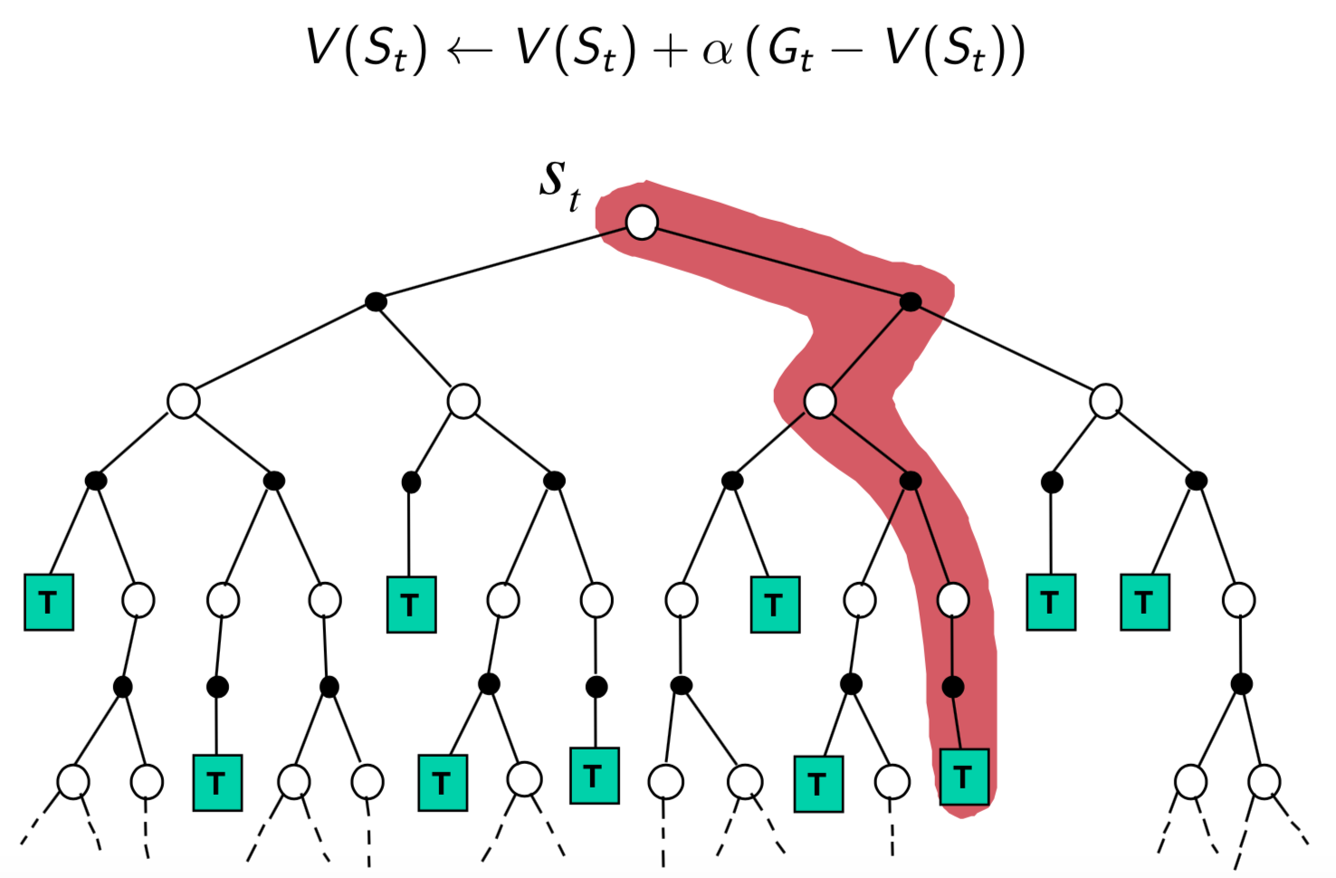
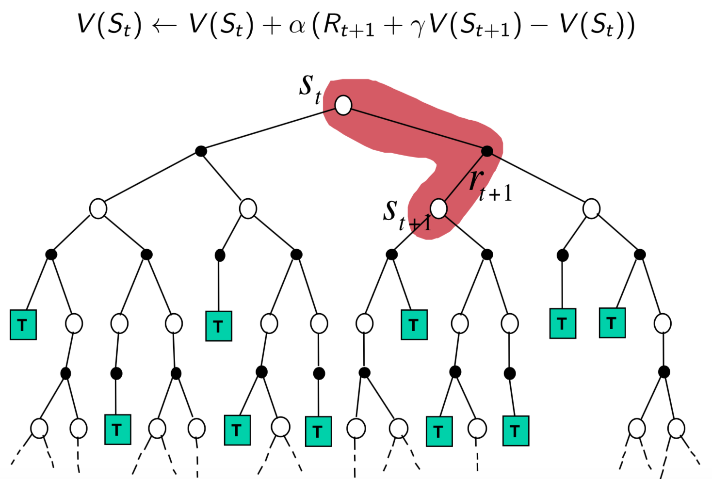
Pros and Cons of MC vs. TD
- TD can learn before knowing the final outcome
- MC must wait until the end of episodes
- TD can learn online after every step
Pros and Cons of MC vs. TD
- TD can learn without the final outcome
- MC can only learn from complete sequences
- When some episodes are incomplete, TD can still learn
- MC only works for episodic (terminating) environments
- TD works in non-terminating environments
Bias/Variance Trade-Off
- Return $G_t=R_{t+1}+\gamma R_{t+2}+...+\gamma^{T-t-1}R_T$ is always an unbiased estimate of $V_\pi(S_t)$
- The true TD target $R_{t+1}+\gamma V_\pi(S_{t+1})$ is an unbiased estimate of $V_\pi(S_t)$
- If we will update $\pi$ slowly along the learning process,
- the TD target $R_{t+1}+\gamma V(S_{t+1})$ becomes a biased estimate of $V_\pi(S_t)$, because
- $V(S_{t+1})$ is a return estimation from the previous $\pi$.
- However, the TD target also has much lower variance than the return $G_t$, because
- the return $G_t$ is from a single rollout, heavily affected by the randomness (actions, transitions, and rewards) in all the future steps;
- whereas the TD target is affected by the randomness in the next one step, and the low variance of the $V(S_{t+1})$ estimation from many historical rollouts.
- the TD target $R_{t+1}+\gamma V(S_{t+1})$ becomes a biased estimate of $V_\pi(S_t)$, because
Pros and Cons of MC vs TD (2)
- MC has high variance, zero bias
- Good convergence properties (even with function approximation)
- Independent of the initial value of $V$
- Very simple to understand and use
- TD has low variance, some bias
- Usually more efficient than MC
- TD(0) converges to $V_\pi(s)$ (but not always with function approximation)
- Has certain dependency on the initial value of $V$
Bellman, or no Bellman, that is the question
- Monte-Carlo sampling and Bellman equation are two fundamental tools of value estimation for policies.
- Each has its pros and cons.
- Based on them, there are two families of model-free RL algorithms, both well developed. Some algorithms leverage both.
- Fundamentally, it is about the balance between bias and variance (sample complexity).
We start from REINFORCE and Deep Q-Learning
- Reason I:
- REINFORCE uses Monte-Carlo sampling
- Deep Q-Learning (DQN) uses Bellman equation
- Reason II:
- REINFORCE only has a policy network
- DQN only has a value network
Taxonomy of RL Algorithms and Examples
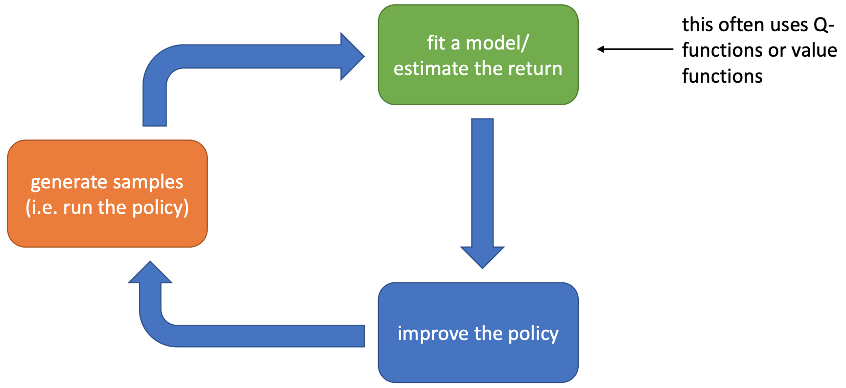
graph TD
l1("RL Algorithms")
l11("Model-Free RL")
l12("Model-Based RL")
l111("MC Sampling
") l112("Bellman based
") l121("Learn the Model") l122("Given the Model") l1111("REINFORCE") l1121("Deep Q-Network") l1-->l11 l1-->l12 l11-->l111 l11-->l112 l12-->l121 l12-->l122 l111-->l1111 l112-->l1121 style l11 fill:#eadfa4 style l111 fill:#eadfa4 style l112 fill:#eadfa4 style l1111 fill:#eadfa4 style l1121 fill:#eadfa4
Q-Learning for Tabular RL
Tabular RL: RL with discrete and finite state space, convenient for algorithm development and convergence analysis
- Suppose we are going to learn the Q-function. Let us follow the previous flow chart and answer three questions:
- Given transitions $\{(s,a,s',r)\}$ from some trajectories, how to update the current Q-function?
- By Temporal Difference learning, the update target for $Q(S,A)$ is
- $R+\gamma\max_a Q(S', a)$
- Take a small step towards the target
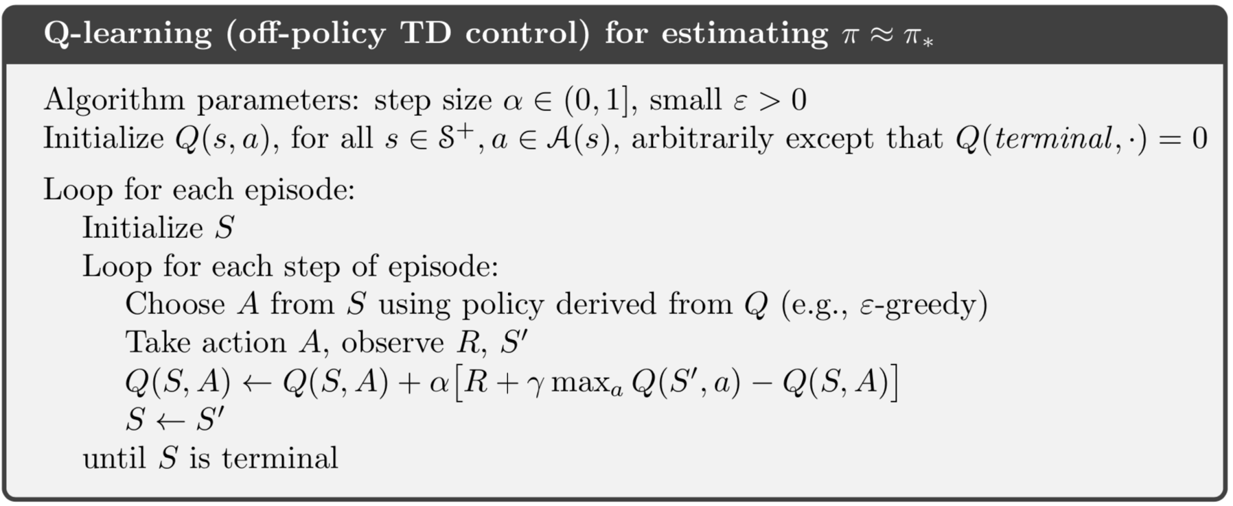
- $Q(S,A)\leftarrow Q(S,A)+\alpha[R+\gamma\max_a Q(S', a)-Q(S,A)]$
- By Temporal Difference learning, the update target for $Q(S,A)$ is
- Given $Q$, how to improve policy?
- Take the greedy policy based on the current $Q$
- $\pi(s)=\text{argmax}_a Q(s,a)$
- Take the greedy policy based on the current $Q$
- Given $\pi$, how to generate trajectories?
- Simply run the greedy policy in the environment.
- Any issues?
Failure Example
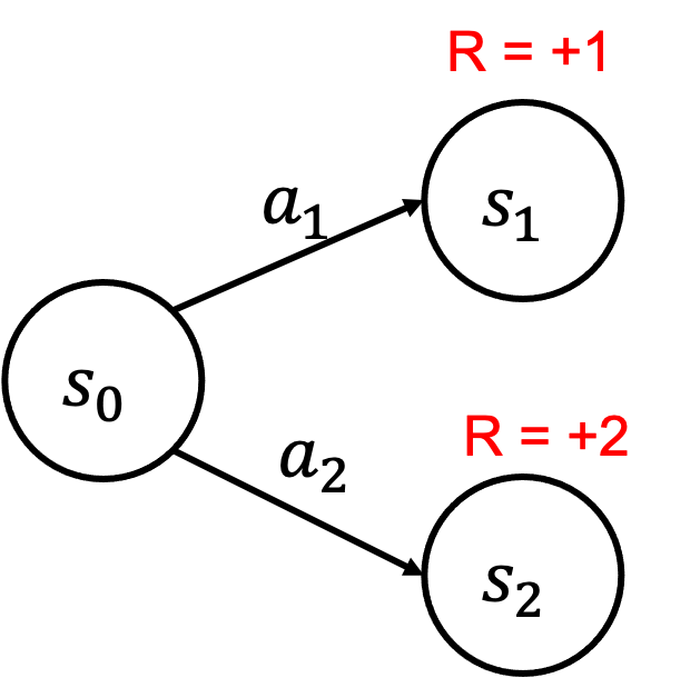
- Initialize Q
- $Q(s_0,a_1)=0,Q(s_0,a_2)=0$
- $\pi(s_0)=a_1$
- Iteration 1: take $a_1$ and update $Q$
- $Q(s_0,a_1)=1,Q(s_0,a_2)=0$
- $\pi(s_0)=a_1$
- Iteration 2: take $a_1$ and update $Q$
- $Q(s_0,a_1)=1,Q(s_0,a_2)=0$
- $\pi(s_0)=a_1$
- ...
- $Q$ stops to improve because the agent is too greedy!
$\epsilon$-Greedy Exploration
- The simplest and most effective idea for ensuring continual exploration
- With probability $1-\epsilon$ choose the greedy action
- With probability $\epsilon$ choose an action at random
- All $m$ actions should be tried with non-zero probability
- Formally, \[ \pi_{\epsilon-Greedy}(a|s)= \begin{cases} \epsilon/m + 1-\epsilon, & \text{if}~~a=\text{argmax}_{a\in\mc{A}}~Q(s,a) \\ \epsilon/m, & \text{otherwise} \end{cases} \]
Exploration vs Exploitation
- Exploration
- finds more information about the environment
- may waste some time
- Exploitation
- exploits known information to maximize reward
- may miss potential better policy
- Balancing exploration and exploitation is a key problem of RL. We use will spend a lecture to discuss advanced exploration strategies.
Q-Learning Algorithm
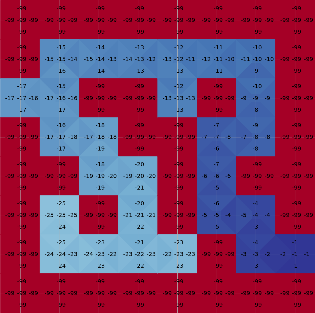
Running Q-learning on Maze
Plot with the tools in an awesome playground for value-based RL from Justin Fu
End
